Safety Stock Calculations

There's several schools of thought on Safety Stock (SS). Some say any stock is a waste, some consider it a necessity for the survival of the business. The point of this article is not to argue that but to offer some options on it, should you choose to maintain safety stock. In this article, we will consider what I call a simple model, a seasonal model and a more advanced model on how to calculate safety stock and look at economic order quantities (EOQ). But without further ado, let's get started.

Basic Requirements

To do any safety stock calculations, you will need to pull several key pieces of information. Mainly, you will need usage history (12 months usage by month), item value, projected sales growth, desired service level and leadtime. The service level should be a value between 0 and 3 where 0 equals 50% service level and 3 equals 100% service level.

Simple Model

This calculation is relatively simple to achieve. You take your 12 month usage and divide by 12, then multiply that by your projected sales growth, then multiply that with how many months of safety stock you wish to hold and then apply a buffer percentage. This will give a crude value that does not take into account any seasonality. If you have huge usage swings, then you best consider the next model. Looks like this:

usage/12 x sales growth x months of stock x buffer percentage

Seasonal Model

In this model, you take your four highest usage months and average them out, multiply by 12 and divide by the days in the year, then multiply by the leadtime in days, then multiply by the sales growth, then multiply by an inventory buffer. Your result will be pretty high because you are averaging your highest months. But you may want to take your safety stock calculations to a higher level, so here's that option.

(4 peak months / 4) x 12) / 365) x leadtime) x sales growth) x buffer percentage

Advanced Model

This model should be combined with an EOQ for best results. The formula uses a service level, which you can define for different parts separately, for example A parts could have a 90% service level since they are super expensive vs C-parts should nearly always be in-stock since they are cheap and therefore should have a 98% service level. The formula multiply's the service factor with 3, then multiply's that by the annual usage divided by working days per year and then that result is to the power of 0.75, then multiplied by the squareroot of the leadtime in days. It looks like this:

3 x service factor x yearly volume / working days per year ^ 0.75 x √leadtime

The result will be tighter than the first two above so be mindful about updating your calculations periodically since your usage may change over time.

Economic Order Quantity

This formula is the Wilson formula and in its simplicity takes the square root of 2 multiplied by annual demand and fixed cost per order and divided by the annual holding cost. It looks like this:

EOQ = √(2 x annual demand x fixed cost per order / holding cost)

Reality Check

Let's put these to the test and see how they fare with some actual data. In the below example, I've calculated the annual cost of each model as expressed in the sum of the holding , ordering and handling cost. For the first two models, there was no EOQ used but orders were placed as they came in so in essence "Lot for Lot". (click on image)

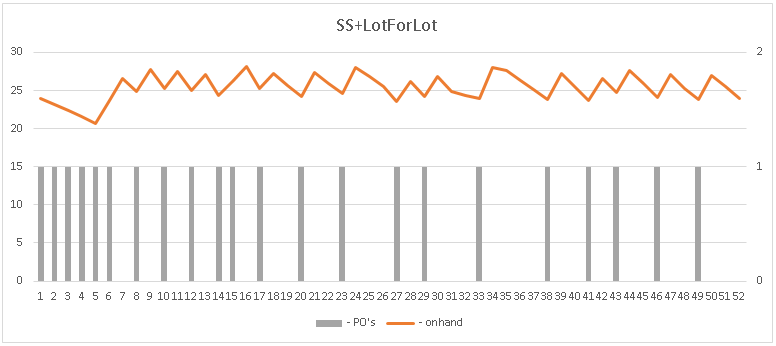
The result shows that the SS+EOQ model gives us the lowest total cost, while the "SS Simple" is twice as costly. The first two create an inventory turnover of 22 while the last maintains a more palatable 7 ITO. Also what should be noted is the cost to replenish stock is significantly lower in the SS+EOQ model. The only difference between the "SS Simple" and "SS Seasonal" is the SS qty. Let's graph what the inventory would look like on a month to month basis between the SS+EOQ vs the SS Seasonal. (click on image)

The left vertical axis is qty onhand portrayed by the orange line and the right axis is the number of orders placed as portrayed by the grey bars. The horizontal axis is weeks in a year. As you can see, the ordering is very frequent which causes higher ordering and handling costs. (click on image)

This shows a much calmer ordering pattern, your peak onhand is higher than the first graph but your safety stock level is lower, so you allow the inventory to move more. This is a more balanced model. Naturally real life will throw some curve balls, like an unexpected customer order or a delayed replenishment shipment but these should not cause stockout's if you used the correct service level value for your product. If you checked my math, you may have noticed that the actual EOQ is 10 but I used 15 to provide more buffer. The result is only a slightly higher inventory holding cost but still significantly lower than the other two models.

Summary

There's several different ways to calculate safety stocks, the above is certainly not a comprehensive guide. Select the one that fits your business model the best and consider the variables. Lastly, you should re-calculate periodically, perhaps quarterly, depending on your market and business fluctuations. Hopefully this short analysis has helped open up safety stock calculations!